Noella Spitz

The Receptive Fields of Convolutional
Neural Networks

One important concept to consider when designing a Convolutional Neural Network (CNN) is the model's receptive field. This is the area of the input region that has an impact on the output features, and therefore the final prediction. If the input image contains an object that is larger than the network's receptive field, the CNN will struggle to correctly identify the objects as it is only working with limited information. This can be illustrated in the image below, where the highlighted rectangle represents a limited receptive field:

It is significantly harder to identify that this object is a car with only that small fragment of the whole image. Furthermore, the issues become more apparent when context matters. For example, if your model's aim is to classify animals in their natural environment, it would need much more contextual clues from the entire image.

For this, there are three main hyperparameters (parameters that define the network structure) to adjust to increase the receptive field of CNNs:

• Increasing the number of convolutional layers
• Subsampling (pooling/strided convolutions)
• Dilated convolutions

In addition to these, padding is also a useful hyperparameter to deal with tensor (multidimensional matrix that holds image/feature map data) shrinkage, which is a consequence of the above methods.

Increasing Layers

Adding more convolutional layers is the most logical way of increasing the network's receptive field. Each convolution condenses the image depending on the filter/kernel size, and the following convolutional layers operate on these condensed versions of the original input. This means that each pixel of the deeper layers contain more and more context, therefore increasing the receptive field.

While this may appear to be a simple solution, increasing the number of layers and therefore the complexity of the network, has significant drawbacks. Adding more layers means that there are more parameters to be trained, which increases training time and computational cost. Furthermore, complex CNN architectures impair the model's ability to generalise, and therefore come with a risk of overfitting, which is where models perform poorly on unseen data (Liu & Zhao, 2022).

Subsampling

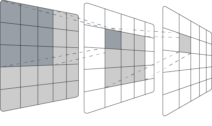
Subsampling means to reduce the spatial resolution, or decrease the number of pixels, in the tensor (Alake, 2020). This increases the network's receptive field by allowing the following convolutions to operate on condensed tensors that provide more context in each unit, an effect similar to adding more convolutional layers (Luo et al., 2016). The most common ways to do this is through pooling or strided convolution.

Pooling layers have two benefits; they lessen computational cost by decreasing the amount of trainable parameters, and extract relevant details while discarding unnecessary ones (Gholamalinezhad et al., 2020). Pooling is typically in the form of average or max pooling, in which the feature map is divided into small regions and either the average value, or highest value, from the region is outputted, respectively.

Stride is a hyperparameter that defines the distance the kernel moves between steps (Yamashita et al., 2018). If the stride is 1 (the default for most operations), the kernel will scan over every element in the feature map, but if the stride is 2, the kernel will skip every other element, moving two spaces at each step. Increasing the stride means that the output shape will be reduced, effectively reducing the spatial resolution.

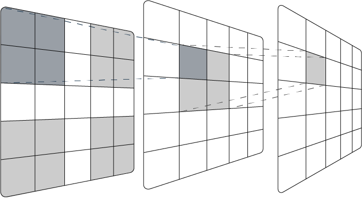
Striding can be included in the convolutional layers, which is referred to as strided convolution. It is a relatively new concept that has received recent attention due to its ability to replace pooling in certain cases whilst increasing accuracy and reducing the memory footprint and network complexity (Ayachi et al., 2020; Springenberg et al., 2014). Strides can also be learned, unlike pooling which is a fixed operation, which provides the opportunity for better accuracy, if there is no concern regarding computational resources.

Pooling and striding can also be used together, as seen in the popular architecture ResNet (He et al., 2015), where pooling is applied sparingly, and instead striding is utilised in the first layers of every convolutional block, to increase the efficiency of the network.

Dilated Convolutions

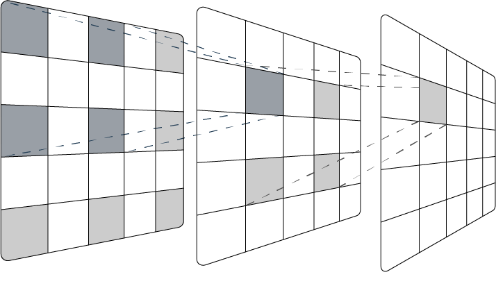
Like strides, the dilation rate is another hyperparameter that can be specified in the convolutional layers. It defines the spacing between the units in a kernel. By spreading out the kernel, the network can widen its receptive field and capture global context without increasing the number of parameters (Sun et al., 2020). As the kernel is more spread out, the resulting output shape is decreased, which allows the network to run more efficiently. However, unlike striding or pooling, there is minimal loss of coverage or resolution, which allows details to be preserved (Li et al., 2021). Additionally, like striding, dilation rate is a hyperparameter that can be learned in order to further optimise the network. All these factors allow dilated convolutions to gain superiority over traditional convolutions, as it effectively enhances model performance without extra computation (Li et al., 2021; Chen et al., 2014)

In tasks where resolution is important, dilated convolutions provide significant advantages. Hamaguchi et al. (2018) proposed a CNN using dilated convolutions for remote sensing imagery with satellites, utilising an approach of decaying dilation rates to maintain the local features of the crowded satellite images. Li et al. (2018) developed a CNN for crowd flow monitoring, which typically involves highly-congested scenes. The model utilised dilated convolutions, omitting pooling completely, and achieved 47.3% lower mean absolute error than state-of-the-art methods.

Padding

After the input has undergone convolutions or subsampling, especially with the introduction of striding or dilation, the resulting output has a reduced size. In order to effectively design a CNN, the changes in the tensor shape must be monitored and understood. The relationship between the hyperparameters and output shape is:

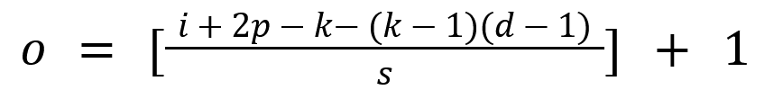
The interactive demonstration below illustrates this tensor shrinkage caused by dilation and strides:

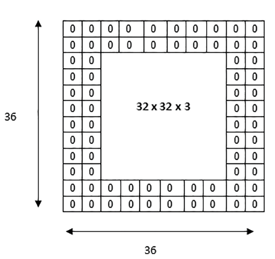
If too much shrinkage is occurring, this can effect the quality of the network's predictions (Fotouhi et al., 2021). Furthermore, as the pixels in the outer edges are only passed by the filter in one path, the information they provide is lost. Padding is an additional hyperparameter that adds a border of zeros around the tensor, to ensure that the outer pixels are propagated to the output as equally as the central pixels, and reduce shrinkage.

Padding also presents other utilities; within the receptive field, research has shown that there exists a phenomenon called the 'effective receptive field', which describes how the most impactful pixels are the ones in the centre of the receptive field. Central pixels have the most paths to propagate to the output, and the impact of each pixel decays the further away it is from the middle, similar to a Gaussian distribution (Luo et al., 2016). If outer pixels are empirical to the task, decreasing this Gaussian effect is important, and this can be done through applying padding or increasing the dilation rate.

Calculating Receptive Field Size

The expression for calculating receptive field size, as a function of hyperparameters, derived by Araujo et. al (2019) is:

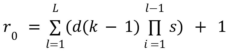
The interactive element below illustrates the receptive field as the hyperparameters are adjusted, applying the equation seen in (2):

As the interactive demonstration illustrates, strides provide the greatest increase in receptive field, however they should be used sparingly as they result in a drastic reduction of the output shape (1). Furthermore, as the number of layers is increased, the number of parameters does as well, and therefore the amount of required computation, which ideally should be minimised.

Significance of the Receptive Field

The receptive field is important in nearly every application of a CNN, however certain tasks may require more attention to this aspect. For CNNs utilised in medical applications, having a receptive field that can capture the entirety of the input image is imperative. In medical image segmentation, a computer vision task that detects the areas of interest in an image to assist in diagnosis, every pixel has to be processed equally to avoid missing important information that could be key to treatment (Alahmadi, 2022). This is also the case for ECG signal analysis, or any biological signal processing task, as each value of a signal has equal importance (Feyisa et al., 2022). In these situations, where errors can have detrimental consequences, the receptive field should be understood and always be taken into account.

References

Alahmadi, M.D. (2022) Medical Image Segmentation with Learning Semantic and Global Contextual Representation. Diagnostics (Basel), 12(7), 1548.
Alake, R. (2020) (You Should) Understanding Sub-Sampling Layers Within Deep Learning. URL: https://towardsdatascience.com/you-should-understand-sub-sampling-layers-within-deep-learning-b51016acd551 [20 March 2023]
Araujo, A., Norris, W. & Sim, J. (2019) Computing Receptive Fields of Convolutional Neural Networks. Distill, 00021
Ayachi, R., Afif, M., Said, Y. & Atri, M. (2020) Strided Convolution Instead of Max Pooling for Memory Efficiency of Convolutional Neural Networks. In: Bouhlel, M.S. & Rovetta, S. (ed.) Proceedings of the 8th International Conference on Sciences of Electronics, Technologies of Information and Telecommunications Vol 1, Manhattan: Springer Cham. pp. 234-243
Chen, L.-C., Papandreou, G., Kokkinos, I., Murphy, K. & Yuille, A. (2022) DeepLab: Semantic Image Segmentation with Deep Convolutional Nets, Atrous Convolution, and Fully Connected CRFs. IEEE Transactions on Geoscience and Remote Sensing, 40(4), pp. 834-848
Feyisa, D.W., Debelee, T.G., Ayano, Y.M., Kebede, S.R. & Assore, T.F. (2022) Lightweight Multireceptive Field CNN for 12-Lead ECG Signal Classification. Computational Intelligence and Neuroscience, 8413294
Fotouhi, S., Pashmforoush, F., Bodaghi, M. & Fotouhi, M. (2021) Autonomous damage recognition in visual inspection of laminated composite structures using deep learningAutonomous damage recognition in visual inspection of laminated composite structures using deep learning. Composite Structures, 268, 113960.
Gholamalinezhad, H. & Khosravi, H. (2020) Pooling Methods in Deep Neural Networks, a Review. ArXiv, abs/2009.07485.
Hamaguchi, R., Fujita, A., Nemoto, K., Imaizumi, T. & Hikosaka, S. (2018) Effective Use of Dilated Convolutions for Segmenting Small Object Instances in Remote Sensing Imagery. 2018 IEEE Winter Conference on Applications of Computer Vision (WACV), pp. 1442-1450.
He, K., Zhang, X., Ren, S. & Sun, J. (2015) Deep Residual Learning for Image Recognition. ArXiv, abs/1512.03385.
Li, B., Hua, Y., Liu, Y. & Lu, M. (2021) Dilated Fully Convolutional Neural Network for Depth Estimation from a
Liu, J. & Zhao, Y. (2022) Improved generalization performance of convolutional neural networks with LossDA. Applied Intelligence.
Li, Y., Zhang, X. & Chen, D. (2018) CSRNet: Dilated Convolutional Neural Networks for Understanding the Highly Congested Scenes. 2018 IEEE/CVF Conference on Computer Vision and Pattern Recognition (CVPR), pp. 1091-1100.
Luo, w., Li, Y., Urtasun, R. & Zemel, R. (2016) Understanding the Effective Receptive Field in Deep Convolutional Neural Networks. 29th Conference on Neural Information Processing Systems. Barcelona, Spain, Dec. 5 - 10.
Rosen, J. (2021) [Photograph]. Unsplash
Springenberg, J.T., Dosovitskiy, A., Brox, T. & Riedmiller, M. (2014) Striving for Simplicity: The All Convolutional Net. ArXiv, abs/1412.6806.
Sun, W., Zhang, X. & He, X. (2020) Lightweight image classifier using dilated and depthwise separable convolutions. Journal of Cloud Computing, 9, 55.
Single Image. Advances in Science, Technology and Engineering Systems Journal, 6(2), pp. 801-807.Traoré, B.B., Kamsu-Foguem, B. & Tangara, F. (2018) Deep convolution neural network for image recognition. Ecological Informatics, 48, pp. 257-268.
Yamashita, R., Nishio, M., Do, R.K.G. & Togashi, K. (2018) Convolutional neural networks: an overview and application in radiology. Insights into Imaging, 9, pp. 611-629.